Investigating the Absorption of Radiation in Matter using G-M Counter

 

Abstract

In this experiment you will study different phenomena related to the polarization of photons. This experiment includes: The study of the effects of two polarizers on the transmission intensity of photons. The effect of a polarizer inserted between two crossed polarizers on the transmission intensity of photons. The effect of a polarizer on the transmission of circular polarization of photons. The effect of a circular polarizer inserted between two crossed polarizers on the transmission of photons.

Introduction

The nature of light

There has always been disagreement over the nature of light since the seventeenth century. Newton and his supporters used to say that the nature of light is a particle. This belief prevailed for a period of time. After that, the wave theory appeared, which says that the nature of light is wave, and this view was supported by some experiments, such as the Yang experiment. Then came Maxwell's electromagnetic theory, which deals with light as a wave consisting of an electric field and a magnetic field. Maxwell developed the equations of his famous theory, and this theory achieved great success.

However, with the beginning of the twentieth century, strange phenomena began to appear that were not obey to the classical theory of electromagnetism, such as the phenomenon of photoelectric effect, the Compton phenomenon and others, which led to a reconsideration of the nature of light so that scientists finally came to the conclusion that light has a dual nature as stated in the research published by the French physicist Louis de Broglie.

Energy flow and Poynting vector

It states that the time rate of flow of electromagnetic energy per unit area is given by the vector S, called the pointing vector defined as the cross product of the electric field and magnetic field divided by the vacuum permeability. It equals to the power over area.

In most cases, a time average of the power delivered per unit area is all that is required. This quantity is called intensity, I

The direction of the electric field vector is known as the polarization of the EM wave. Since the polarization supports the wave theory, we should understand it.

Linear Polarization

A polarizer selectively absorbs light or transmit it according to its transmission axis. The state of polarization of light can most easily be tested by a second polarizer which function as analyzer.

Linear polarization

The intensity I of polarized light after passing through a polarizing filter can be detected by Mauls’ Law:

I=I₀cos²θ

Circular, Elliptical Polarization and Quarter wave plate (QWP)

Circularly polarized light can be produced by introducing a phase shift of pi/2 between two orthogonal components of linearly polarized light. One device for doing this is known as quarter wave plate. These plates are made of doubly refracting transparent crystals, such as calcite of mica. Doubly refracting crystals have the property that the index of refraction differs for different directions of polarization.

The orientation of the quarter-wave plate is defined by the angle (Pi) between the transmission axis of the polaroid and the fast axis of the quarter-wave plate. By choosing ɵ to be 45 degrees, the light entering the quarter-wave plate can be resolved into two orthogonal linearly polarized components of equal amplitude and equal phase. Upon emerging from the quarter-wave plate, these two components are out of phase by Pi /2. Hence the emerging light is circularly polarized.

Polarized light can be represented by a Jones vector, and linear optical elements are represented by Jones matrices. When light crosses an optical element the resulting polarization of the emerging light is found by taking the product of the Jones matrix of the optical element and the Jones vector of the incident light. Note that Jones calculus is only applicable to light that is already fully polarized. Light, which is randomly polarized, partially polarized, or incoherent must be treated using Mueller calculus.

Methodology

Apparatus

The apparatus consists of the following elements and devices, mentioned in order as will be seen in the experimental setup Figure below:

*Source: a 6 V AC incandescent lamp with housing.

*A condenser lens to focus the light as will be discussed in the procedure.

* An iris to limit the stray light

* An additional lens may be used to obtain a parallel light beam. Another lens to focus the parallel light beam on the photocell.

* A glass filter to get a band of light preferably as small as possible.

* Optical elements (polarizers, Quarter wave plate, and neutral density filters).

* A photocell to detect the light photons.

*An ammeter which can detect currents as low as few microamps.

* An optical bench to hold all the optical elements and devices.

Procedure

Part1: Using one polarizer

We turn on the light and control the Iris radius, then we put the polarizer and changed its angle from -90 to 90 and read the intensity from the micrometer.

Part2: Using two polarizers.

We set the first polarizer at angle 0 degree and changed the second one angle from -90 to 90 and recorded the intensity.

Part3 : 3 Polarizers

We arranged the 3 polarizers parallel to each other and set the 1st and the 3rd one at zero angle while changing the 2nd one angle from -90 to 90 degree.

Part4: 3 Polarizers

As the same setup in part3 but the 2nd one is changing from -90 to 90 and the third one stetted at zero angle.

Part5 : 2 Polarizers and QWP

At this part we replaced the 2nd polarizer with a QWP changing his angle from 0 to 180, the first polarizer at 0 degree, and the second at 90.

Part6: 2 Polarizers and QWP

Same setup as part5 but we set QWP at angle 45 and changed the 2nd polarizer angle from    -90 to 90.

Data Analysis

Part 1

Is = 20 𝝁A

I when using one polarizer= I₀/2= 10𝝁A

                  Table (1)

θ	I(10^-6) A	I/I0
-90	10.7	0.535
-80	10.8	0.54
-70	9.9	0.495
-60	9.9	0.495
-50	10.6	0.53
-40	10.6	0.53
-30	10.1	0.505
-20	10.4	0.52
-10	10.3	0.515
0	10.3	0.515
10	10.3	0.515
20	10.3	0.515
30	10.4	0.52
40	10.4	0.52
50	10.5	0.525
60	10.6	0.53
70	10.6	0.53
80	10.7	0.535
90	10.7	0.535

Figure1: shows the relation between the intensities ratio and the angle using one polarizer.

For one polarizer, the light is linearly polarized with jones vector = 

<I> = 9.905

<I> Theoretical = I₀/2 = 10 𝝁A

Part 2

Using Two polarizers

First polarizer is fixed at 0 degree. The second polarizer is varied (-90- 90)

                  Table (2) 

θ	I(10-6) A	I/I0	Cos2 θ
-90	0	0	0
-80	0.4	0.02	0.030154
-70	1	0.05	0.116978
-60	1.9	0.095	0.25
-50	3	0.15	0.413176
-40	4	0.2	0.586824
-30	4.9	0.245	0.75
-20	5.6	0.28	0.883022
-10	6.1	0.305	0.969846
0	6.3	0.315	1
10	6.2	0.31	0.969846
20	5.9	0.295	0.883022
30	5.3	0.265	0.75
40	4.3	0.215	0.586824
50	3.3	0.165	0.413176
60	2.3	0.115	0.25
70	1.2	0.06	0.116978
80	0.6	0.03	0.030154
90	0	0	0

^{Figure2: shows the relation between the intensities ratio and the angle using 2 polarizers.}

^{Figure3: shows the relation between the intensities ratio and the square of the angle using two polarizers.}

The slope must equal to 1 between cos²θ and I/I₀ theoretically but we obtained 0.3083 experimentally.

The linear polarized light emerges from the first polarizer.

The Jone matrix of polarizer with transmission axis at angle θ with horizontal.

J.V= A , Where A is the Jone matrix representing the final emerging light.

The flux intensity

Read alsoBeta Spectroscopy Experiment

Read alsoPhoton Polarization Experiment

Read alsoMillikan Oil Drop Experiment

Read alsoKerr Effect Experiment

Part 3

Polarizer inserted between two parallel ones.

θ	I(10^-6) A	(cosθ)^4	I/I0
-90	0	0	0
-80	0.4	9.09*10^-4	0.02
-70	0.5	0.136838	0.025
-60	0.8	0.0625	0.04
-50	1.4	0.17071	0.07
-40	2.4	0.344363	0.12
-30	3.2	0.5625	0.16
-20	4.2	0.779728	0.21
-10	4.8	0.940601	0.24
0	6	1	0.3
10	4.8	0.940601	0.24
20	4	0.779728	0.2
30	3	0.5625	0.15
40	2	0.344363	0.1
50	1.2	0.17071	0.06
60	0.7	0.0625	0.035
70	0.5	0.136838	0.025
80	0.3	9.09*10^-4	0.015
90	0	0	0

Figure4: shows the relation between the intensities ratio and the angle using 3 polarizers.

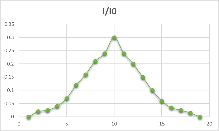
Figure5: shows the relation between the intensities ratio and cosine to the power 4 of the angle using 3polarizers.

Part 4

Polarizer inserted between two crossed  ones.

θ	I(10^-6) A	(cosθ)^4	I/I0
-90	0.3	0	0.015
-80	0.5	9.09*10^-4	0.025
-70	0.8	0.136838	0.04
-60	1.2	0.0625	0.06
-50	1.45	0.17071	0.0725
-40	1.4	0.344363	0.07
-30	1.2	0.5625	0.06
-20	0.7	0.779728	0.035
-10	0.4	0.940601	0.02
0	0.3	1	0.015
10	0.5	0.940601	0.025
20	0.9	0.779728	0.045
30	1.3	0.5625	0.065
40	1.7	0.344363	0.085
50	1.6	0.17071	0.08
60	1.4	0.0625	0.07
70	0.9	0.136838	0.045
80	0.5	9.09*10^-4	0.025
90	0.1	0	0.005

 Figure6: shows the relation between the intensities ratio and the angle using 3 polarizers. Figure6: shows the relation between the intensities ratio and the angle using 3 polarizers.

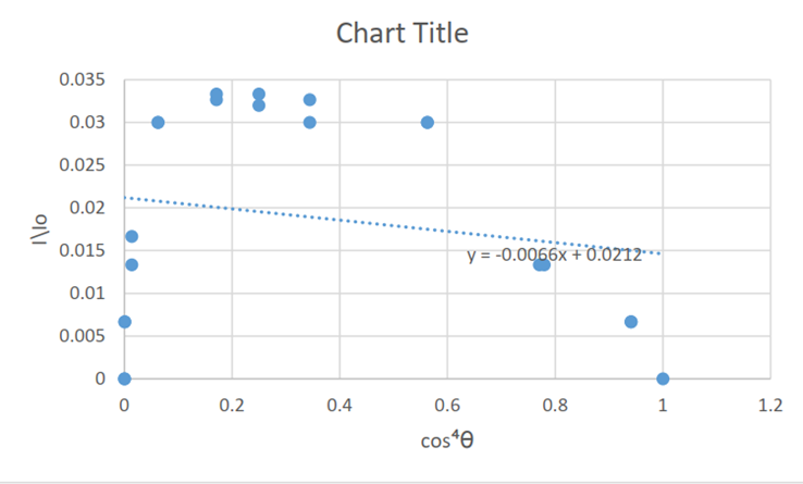
Figure7: shows the relation between the intensities ratio and cosine to the power 4 of the angle while using 3polarizers.

P.E = │(0.5-(-0.066))/0.5│ = 113%

Part 5

QWP inserted between two crossed  Polarizer.

θ	I(10^-6) A	I/I0
0	0.1	0.005
10	0.3	0.015
20	1	0.05
30	1.6	0.08
40	2	0.1
50	1.85	0.0925
60	1.4	0.07
70	0.7	0.035
80	0.2	0.01
90	0.1	0.005
100	0.4	0.02
110	1	0.05
120	1.7	0.085
130	2	0.1
140	2.05	0.1025
150	1.5	0.075
160	0.8	0.04
170	0.3	0.015
180	0.1	0.005

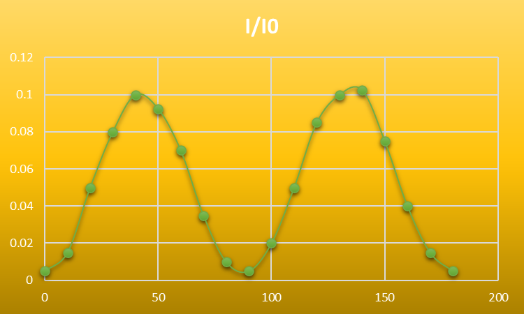
       Figure8: shows the relation between the intensities ratio to the angle while using  polarizers and QWP.

Jones matrix of QWP at any angle is :

Part 6

Two polarizers the first with 0 angle, second varies and QWP at 45 degree.

θ	I(10^-6) A	I/I0
-90	2	0.1
-80	2	0.1
-70	2.1	0.105
-60	2.3	0.115
-50	2.6	0.13
-40	2.8	0.14
-30	3.1	0.155
-20	3.3	0.165
-10	3.4	0.17
0	3.5	0.175
10	3.5	0.175
20	3.3	0.165
30	3.2	0.16
40	2.9	0.145
50	2.6	0.13
60	2.4	0.12
70	2.2	0.11
80	2	0.1
90	2	0.1

   Figure9: shows the relation between the intensities ratio and the angle using polarizers and QWP.

Conclusion

§       The light propagates as a wave and interact with matter as a particle (particle-wave duality).

§       Any interaction of light with matter whose optical properties are asymmetrical along directions transverse to the propagation vector provides a means of polarizing light.

§       In this experiment we use both the quantum theory and the classical theory of light.

§       The light is a transverse electromagnetic wave which consist of electric and magnetic components which are both perpendicular on the direction of propagation.

References

1- Third Edition, Introduction to Optics, PEDROTT.

2- Practical physics (0342411) manual.

3- https://tikz.net/files/optics_polarization-002.png