Investigating the Absorption of Radiation in Matter using G-M Counter

 

Abstract

In this experiment, we shall investigate the characteristics of Geiger-Mueller counter (operating plateau, dead time), inverse square law  the absorption of gamma rays in matter and determine the linear and mass absorption coefficients of radiation in a number of materials, the absorption of beta rays in aluminum and determine the maximum energy of emitted beta particles.

Introduction

A. Particle Detectors

A particle moving in a gas loses its energy through interaction with the gas molecules, primarily through the ionization of the gas molecules. Thus, a particle makes several electron-ion pairs as it moves through the gas. For example, a low-ionizing particle such as β particle could produce few tens of pars, where as a heavily ionizing particle such as α particle could produce several tens of thousands (104 – 105) of pairs.

 If the electrons from the ionization process are collected by an anode, they produce a pulse that can be detected. Particle detectors are designed to respond to a single ionizing particle or quantum of radiation. A typical detector consists of metallic cylinder, which contains appropriate mixture of ionizable gases, and a fine wire (the anode) fixed at its axis. As a particle inters the detector, it produces a number of electron-ion pairs depending on the nature and energy of the incoming particle. 

When a potential difference is established between the anode and wall of the cylinder (cathode), the electrons are collected at the anode and a pulse is produced which height is proportional to the number of electron-ion pairs as shown in Fig. 1. In region I, the voltage is not high enough to collect all electrons, and a competition between recombination and electron collection leads to a collected number less than that produced by ionization. In region II, the potential is high enough that all ionized pairs are collected, independent of the value of the applied potential. In this horizontal region, the pulse height is proportional to the number of initial ionization pairs. This is the region for the operation of the ionization chamber. In region III, electrons from the primary ionization acquire enough energy to ionize other molecules and gas amplification results.

Figure 1: The number of electron-ion pairs collected as a function of applied  potential.

 

An avalanche occurs in this region where the number of collected pairs increases exponentially. In the first part of this region (the proportional counter operation region) the curves for the low and high ionizing particles are parallel and the number of collected pairs is proportional to the number of primary pairs. In the second part of region III (the region of limited 50 proportionality), the higher the number of ion pairs is, the slower is the rise of the curve due to higher positive space charge which inhibits avalanche.

In region IV, the number of collected pairs is independent of the number of primary electron-ion pairs, and the total number of collected pairs is determined by the characteristics of the detector tube and the experimental set up. In this region, a high pulse appears, signaling the arrival of one ionizing particle or  quantum, regardless of its nature the number of primary pairs it produces. This is the Geiger-Mueller counter operation region. Beyond this region, the count rate increases indefinitely, signaling the region of continuous discharge across the tube (do not go into this discharge region in operating the tube).

Geiger counter

According to the previous discussion, the G-M counter is most suited for the detection of low ionizing particles and quanta, such as electrons and gamma rays. However, this counter does not reveal information on the nature of the ionizing agent. A schematic diagram of the G-M counter is shown in Fig. 2, where the collected electrons at the anode appear as charge on the capacitor, which is discharged through a resistance RL producing a voltage pulse that can be detected.

The efficiency of the Geiger counter is rather high (>90%) for charged particles, but is rather low (1-2%) for photons. Thus, accurate determination of the activity of a radioactive source by a Geiger counter involves some calculations and estimations. However, the flatness of the plateau is a measure of the efficiency of the tube.

B. Dead Time

When an avalanche of electron-ion pairs is produced in a G-M counter due to passage of a particle or a photon, electrons are collected at the anode producing a pulse, and positive ions are neutralized at the wall of the grounded tube. This process takes time, during which the tube is inoperative (cannot detect incoming particles or photons). This time is thus termed “dead time”. The loss in counts due to dead time is thus more for higher number of counts. Thus, if we have two sources, which give count rates R1 and R2 when placed in front of the tube separately, and a count rate R12 when placed together in their respective positions, the dead time of the tube is given by equ.3.

C. Absorption of γ-rays

When γ-rays go through an absorbing medium, they get absorbed by the different processes through which they interact with matter, such as Compton scattering, photoelectric, and pair production interactions. If the thickness of the absorbing material is x, the transmitted intensity of radiation is then given by equ.5.

D. Absorption of β-Particles

When a charged particle, such as electron, inters a region of matter, it interacts with the matter, losing its energy primarily through ionization of the matter atoms . Beta particles emitted from a nucleus has a distribution of energies with a maximum energy that can be determined from the range of the particles in a given material. The range (D) of the particle in the material is the total thickness of material the particle traverses before losing its energy completely. 

The range of a charged particle in a given material depends on the nature of the particle, and the physical properties of that material. Thus, extensive work had been carried out for different particles and different absorbers. Also, various empirical formulas have been developed for the range of a charged particle in a material. For example for electrons with energy E > 0.8 MeV, Feather’s equation gives the range in density thickness (g/cm2) of aluminum (equ.8).

Methodology

A. Characteristics of Geiger counter

1. Make sure that the potential across the G-M tube is zero. Place a radioactive source at a suitable distance from the tube (about 5 cm), and switch on the power. 54
2. Slowly increase the potential difference at the anode until the count rate is detectable (this occurs between 360 and 400 V). Then record the number of counts per 100 s against voltage in steps of 20 V. Watch the increase in counting with increasing voltage carefully, and do not go into the discharge region (above 600 V for some tubes). Also, watch for overflow of counts and account for the number of overflows, or select the (x 10) scale.
3. Plot a quick relation between the count number and voltage to determine the plateau region and the operating voltage.

B. Dead Time

1. Set the G-M tube at the operating voltage.
2. Make sure to have well defined positions for two sources about 5 cm from the window of the tube. Do not change or disturb these positions during the following experiment.
3. Place the first source in place, and record the number of counts N1 in 100 s. Repeat the measurement three times and take the average.
4. Carefully place the second source in position without disturbing the first. Record in 100 s the combined count N12. Repeat three times and take the average.
5. Now carefully remove the first source without disturbing the setup. Make a 100 s count N2, repeat three times and take the average.

C. Absorption of γ-rays

1. Set the G-M tube at the operating voltage.
2. Place the 137Cs source about 5 cm from the tube window, and count for 100 s. Record the number of counts for “zero” absorber thickness. If the number of counts is low (hundreds of counts), take 4 measurements of the count and take the average.
3. Place a thin lead sheet (1-3 mm thick) between the source and tube window and repeat the measurement for the same period of time as in step 2. Record the number of counts (4 times if the count rate is low) and the thickness of the lead sheet.
4. Repeat the measurement of the number of counts over the same period of time for additional
thick sheets of lead (about 6.6 mm each) until the observed count rate is less than 25% of its original value (with no absorber), and record the observed count and the total thickness of lead sheets.
5. Repeat the experiment using Cu sheets (1mm thick each) as absorber material. For this experiment, you may need to increase the distance between the source and detector widow up to about 6 cm to allow space for absorber sheets.
6. Repeat the above procedure using or 60Co source.
7. Make three measurements of the background count for the same counting time and take their average. This should be subtracted from the number of counts to obtain the corrected count.

D. Absorption of β-rays in Aluminum

1. Set the G-M tube at the operating voltage.
2. Place a β source (90Sr) about 4 cm from the tube window, and count for 100 s. Record the number of counts for “zero” absorber thickness.
3. Place a thin aluminum foil (0.5 mm) between the source and tube window and repeat the measurement for the same period of time as in step 2. Record the number of counts and the thickness of the aluminum foil.
4. Repeat the measurement of the number of counts over the same period of time for different additional foils of Al, and record the observed count and the total thickness of Al foils.

Formalism

Data Analysis

-Absorption of γ-rays:

1. Lead (Pb):

Density of Pb=11.35 g/cm³.

Table 1 below contains the number of counts N for γ radiation, using different thicknesses x of lead as an absorber, and the density thickness 𝜉 (= ρχ):

Ln(N)	Density Thickness "𝝃" (g/cm2)	Number of counts "N"	Thickness "x" (mm)
6.364751	0	581	0
6.214608	1.135	500	1
6.025866	8.7395	414	7.7
5.583496	12.939	266	14.4
5.411646	23.9485	224	21.1
5.153292	31.553	173	27.8

Figure 2 below plots Ln(N) versus the density thickness 𝜉:

From Figure 2, the equation of the straight line is:

ln N = -0.0372𝜉  + 6.2778

 

We want to find the half value layer density thickness 𝜉 1/2, and then the half value layer thickness χ1/2.

From Equation

Read alsoDiffraction Grating Spectrometry Experiment

Read alsoElectron Diffraction Experiment

Read alsoBeta Spectroscopy Experiment

Read alsoPhoton Polarization Experiment

ln N = ln N0  - μ𝜉 .... (7)

 we see that the intercept is Ln N0  , so:

ln N = -0.0372𝜉 + ln N0 

Substituting N = (1/2)N0 :

ln(N0 /2) =  -0.0372𝜉1/2 + ln N0

 ln N0 - ln2 = -0.0372𝜉1/2 + ln N0

Eliminating ln N0 from both sides:

- ln2 = -0.0372𝜉1/2

0.0372𝜉1/2 = ln2 / 0.0372

 And then we find  𝜉1/2 :

𝜉1/2 = 18.63 g/cm^2

Using this result and equation

  𝜉1/2 = ρχ1/2

χ1/2 = 𝜉1/2 / ρ  = 18.63 / 11.35 = 1.64 cm = 16.4 mm

χ1/2  = 16.4 mm 

From equation (7) , we see that the slope is minus the mass absorption coefficient: 

slope = - μ = - 0.0372

Then:

 μ = 0.0372 cm^2 / g

And from this result we can calculate the linear absorption coefficient k using equation

μ = k / ρ 

k = μ  * ρ = (0.0372)*(11.35) = 0.42222 cm^-1

k =  0.42222 cm^-1

Figure 3 below plots Ln(N) versus the thickness x:

 From Figure 3, the equation of the straight line is:

ln N = -0.0428x + 6.3053

From equation 

ln N  = ln N0  - k x .... (6)

, we see that the slope is minus the linear absorption coefficient:

Slope = - k = - 0.0428

Then: 

k = 0.0428 mm^-1  =  0.428 cm^-1 

And from this result we can calculate the mass absorption coefficient μ using equation

μ = k /  ρ ... (4)

μ = k /  ρ = 0.428 / 11.35 = 0.0377 cm^2 / g

 μ = 0.0377 cm^2 / g

1. Copper (Cu):

Density of Cu=8.9 g/cm³.

Table 2 below contains the number of counts N for γ radiation, using different thicknesses x of copper as an absorber, and the density thickness 𝜉(= ρχ): 

Ln(N)	Density Thickness "𝝃" (g/cm2)	Number of counts "N"	Thickness "x" (mm)
6.364751	0	581	0
6.25575	4.45	521	5
5.996452	8.9	402	10
5.961005	13.35	388	15
5.755742	17.8	316	20

Figure 4 below plots Ln(N) versus the density thickness 𝜉:

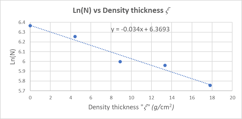
From Figure 4, the equation of the straight line is:

ln N = -0.034𝜉  + 6.3693

We want to find the half value layer density thickness 𝜉1/2, and then the half value layer thickness χ1/2.

From Equation (7) , we see that the intercept is Ln (N0) , so: 

ln N = -0.034𝜉 + ln N0

Substituting N = (1/2)N0 :

ln(N0 /2) =  -0.034𝜉1/2 + ln N0

 ln N0 - ln2 = -0.034𝜉1/2 + ln N0

Eliminating ln N0 from both sides:

- ln2 = -0.034𝜉1/2

𝜉1/2 = ln2 / 0.034

 And then we find  𝜉1/2 :

𝜉1/2 = 20.39 g/cm^2

Using this result and equation

  𝜉1/2 = ρχ1/2

χ1/2 = 𝜉1/2 / ρ  = 20.39 / 8.9 = 2.29 cm = 22.9 mm

χ1/2  = 22.9 mm 

From equation (7) , we see that the slope is minus the mass absorption coefficient: 

Slope = - μ = - 0.034

Then:

 μ = 0.034 cm^2 / g

And from this result we can calculate the linear absorption coefficient k using equation

μ = k / ρ 

k = μ  * ρ = (0.034)*(8.9) = 0.3026 cm^-1

k =  0.3026 cm^-1

Figure 5 below plots Ln(N) versus the thickness x:

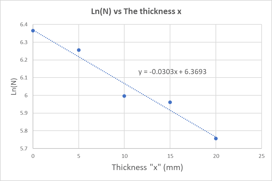
 From Figure 5, the equation of the straight line is:

ln N = -0.0303x + 6.3693

From equation 

ln N  = ln N0  - k x .... (6)

, we see that the slope is minus the linear absorption coefficient:

Slope = - k = - 0.0303

Then: 

k = 0.0303 mm^-1  =  0.303 cm^-1 

And from this result we can calculate the mass absorption coefficient μ using equation

μ = k /  ρ ... (4)

μ = k /  ρ = 0.303 / 8.9 = 0.03404 cm^2 / g

 μ = 0.03404 cm^2 / g

-Absorption of β-rays in Aluminum:

Density of Al=2.7 g/cm³.

Table 3 below contains the number of counts N for β radiation, using different thicknesses x of aluminum as an absorber, and the density thickness 𝜉(= ρχ):

Ln(N)	Density Thickness "𝝃" (g/cm2)	Number of counts "N"	Thickness "x" (mm)
10.30025	0	29740	0
9.541082	0.135	13920	0.5
8.891512	0.27	7270	1
7.986165	0.405	2940	1.5
7.17012	0.54	1300	2
6.173786	0.675	480	2.5
5.010635	0.81	150	3
4.60517	0.945	100	3.5
4.189655	1.08	66	4
4.174387	1.215	65	4.5
4.174387	1.35	65	5
3.970292	1.485	53	5.5
3.931826	1.62	51	6
4.174387	1.755	65	6.5
3.951244	1.89	52	7

Figure 6 below plots Ln(N) versus the density thickness 𝜉:

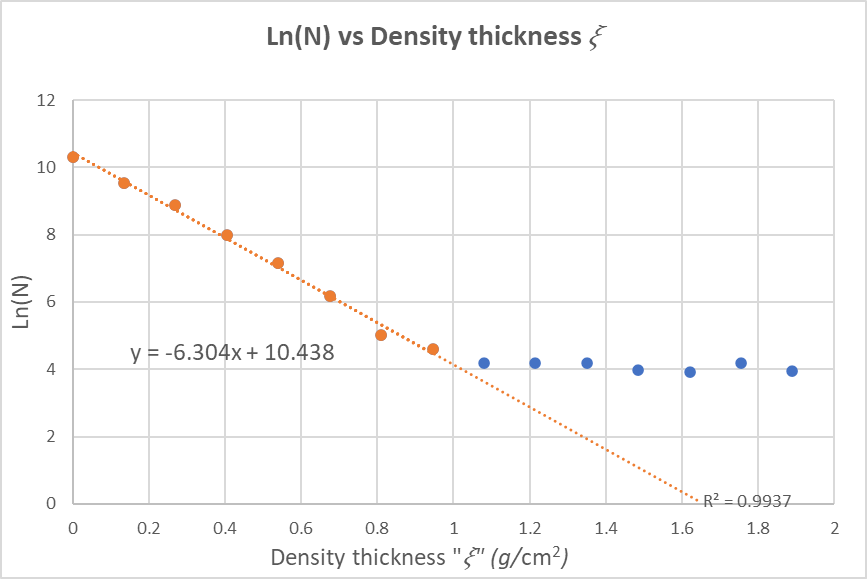
From Figure 6 above, the range D(g/cm²) of electrons in Al, is the interception of the line with the x-axis (y=0):

0 = -6.304D + 10.438

6.304D = 10.438 

D = 10.438 / 6.304 = 1.656 cm^2 / g

D = 1.656 cm^2 / g

 to find the energy of electrons E:

D (g / cm^3) = 0.412E^(1.265 0.0954lnE)

1.656 = 0.412E^(1.265 0.0954lnE)

Solving for E :

E = 3.35 MeV

Using Feather's equation,

D (g / cm^3) =0.543E - 0.160

1.656 = 0.543E - 0.160 

Solving for E:

E = 3.34 MeV

Conclusion 

ln this report we first studied the characteristic of the Geiger counter. The Geiger counters properties are different depending on the age of the tube, its dimensions the gas it contains and many other systematic properties. These properties determine the value of the operating voltage of the counter. To obtain its value we take counts vs potential and study the plateau region. Also, there is another property that should be taken in account, the dead time where the counter doesn’t operate. By obtaining this time we do a correction to the counts because the dead time, lowers the real value of the counts. We noticed that for high counts dead time correction is significant. 

However for low ones it isn’t, because of the denominator which is (1-R T), so because of very small dead time we need a high number of counts in order for the denominator to effect the value of R0_ We also studied several radiating materials and absorbing materials . Cs emits gamma rays, and we studied the absorption of gamma rays in lead and copper. We found that the absorption coefficient of lead is higher than cooper and so if they are of the same thickness lead absorbs the radiation more than copper. That is why χ1/2 is lower in lead than in copper. These values were obtained by drawing graphs of Ln(count)vs thickness and thickness density. The relation between them is linear with an intercept equal to the number of counts when the thickness is zero.

 ln the last part we studied the beta absorption, our source was 5r 90 and we used aluminum as our absorption material, we notice that aluminums density ls less than lead and copper, however it did absorb most of the radiation with a small thickness and that indicates that beta particles do not have a high ability of penetration. We drew a graph of Ln count vs thickness density and obtained a linear relation from that relation we determined the Range of electrons and that is when an electron loses all its energy this is determined when the count is zero. We found D to equal 1.5 g/cm2 and by feathers equation and empirical formula we found the energy of the electron. The energies differ in both relations because the of the empirical is correct for energies between 0.01 and 2.5 MeV, but our energy was 3.0571 MeV.

References

Practical advanced physics, Sami Mahmoud, University of Jordan, 2012.